What Is the Best Input Pipeline to Train Image Classification Models with tf.keras?
A comparison between Keras’ ImageDataGenerator, TensorFlow’s image_dataset_from_directory and various tf.data.Dataset pipelines
When we start learning how to build deep neural networks with Keras, the first method we use to input data is simply loading it into NumPy arrays. At some point, especially when working with images, the data is too large to fit in memory so we need an alternative to arrays. From my experience, the go-to solution to that problem is to use the tool built into Keras called ImageDataGenerator. This creates a Python generator that feeds the data gradually to the neural network without keeping it into memory. Additionally, it includes data augmentation features that make it a very useful tool.
This could be the end of the story, but after working on image classification for some time now, I found out about new methods to create image input pipelines that are claimed to be more efficient. The goal of this article is to run a few experiments to figure out the best method out there. The main contestants will be:
tf.keras.preprocessing.image.ImageDataGeneratortf.keras.preprocessing.image_dataset_from_directorytf.data.Datasetwith image filestf.data.Datasetwith TFRecords
The code for all the experiments can be found in this Colab notebook.
Experimental setup
To have a fair comparison of the pipelines, they will be used to perform exactly the same task: fine tune an EfficienNetB3 model to classify images in two different datasets. Before describing the datasets, here is the training pipeline that is used, strongly inspired by this tutorial.
This code simply takes a pretrained EfficientNetB3 and adds a classification layer on top of it with the right number of neurons. This model is then trained for 5 epochs with a batch size of 32 with each tested method. The experiments are done on Google Colab, with the hardware available with Colab Pro. The version of TensorFlow used is 2.4.1.
The first dataset used to test the pipelines is a subset of the Open Images Dataset [1] consisting only of fruit images. The second one is the Stanford Dogs Dataset [2–3] with images of various dog breeds. Here is a summary of the two datasets:

The datasets are pretty different since one has a small number of classes with less images that are larger in size. Code to download and prepare these datasets is presented in the colab.


Conclusions
Since the rest of this article spends a good amount of time explaining the different input pipelines and some people may only care about the conclusions, here is a summary of all the experiments:

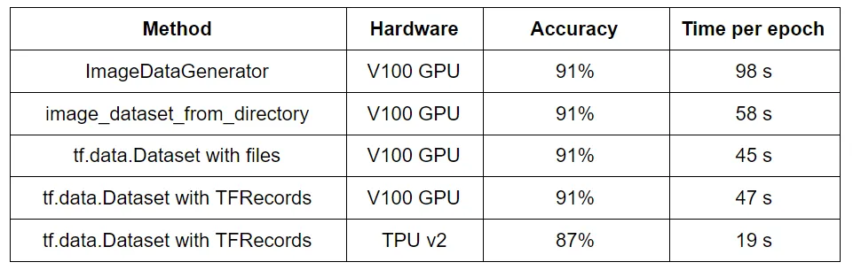
The numbers clearly show that the go-to solution ImageDataGenerator is far from being optimal in terms of speed. The only reason to keep using it could be because of how simple data augmentation is with this method. It is however not that hard to do with the other methods, and could be worth it given the big improvement in speed.
In my opinion, image_dataset_from_directory should be the new go-to because it is not more complicated that the old method and is clearly faster.
Building our own input pipeline using tf.data.Dataset improves speed a bit but is also a bit more complicated so to use it or not is a personal choice.
Concerning TFRecords, it seems that if one is not working with TPUs they are not necessary since working directly with the image files makes no difference in performance.
The optimal solution seems to be using TFRecords with a TPU and given the increase in speed it is worth the extra trouble. The drop in accuracy comes simply from the fact that different hyperparameter combinations are efficient with the TPUs but the tests used the same as the GPU. Using the right hyperparameters lead to similar accuracies than with the other methods.
ImageDataGenerator
Let’s now jump into the details of each method, starting with a review of the reigning champion, which is very simple.
The Keras method takes the data stored into a folder, with each subfolder corresponding to an individual class. In this example, it resizes the images and creates batches automatically. The labels are generated from the subfolder names. The ‘sparse’ format is used to have labels of the form 0,1,2,3,... because the sparse metrics are used in the model building.
The main advantages of this method are its extreme simplicity and the fact that data augmentation can be done simply by specifying the transformations (rotation, flip, zoom, etc) in the arguments.
image_dataset_from_directory
The next option is also pretty simple and is included in Keras as well.
The format of the data is the same as for the first method, the images are again resized and batched, and the labels are generated automatically. There are however no options to do data augmentation on the fly.
The main difference in this method is that the output is not a python generator but a tf.data.Dataset object. This allows it to fit nicely with the rest of the pipelining tools discussed below. For example, a prefetch of the data is done here to help make the calculations faster. Any form of data augmentation done with TensorFlow can be done on this kind of dataset. It is a bit less simple but much more customizable.
tf.data.Dataset
TensorFlow recommends using tf.data when working with the library to achieve optimal performance. This is a set of tools to create a dataset made of tensors, apply transformations to the data and iterate over the dataset to train neural networks. It works with any type of data, like tables, images or text. The data can be imported in multiple ways. The most common ones are NumPy arrays, python generators, CSVs, TFRecords and strings. Much more detail can be found on Tensorflow’s website.
Let’s start by showing the code used for this specific case of image classification, and then explain how it works.
The first step that is done here is to format the data needed correctly before feeding it to TensorFlow. The format that is used here is a filepath and an integer label for each image. This processing is done in lines 19–22. It is extremely important to not forget to shuffle the list of images because the performance of the model would be greatly affected. Trust me…
Note: An alternate method is to directly get the list of files using tf.data.Dataset.list_files . The problem with this is that the labels must be extracted using TensorFlow operations, which is very inefficient. This slows down the pipeline by a lot so it is preferred to get the labels with pure python code.
The labels part is simple because the list of labels is converted to a dataset using the method from_tensor_slices , which converts any tensor-like object (numpy array, list, dictionary). The list of filenames is also converted to a dataset using the same method.
The next step is to apply the parse_image function to the filenames dataset using the map method, which applies a TensorFlow function to all the elements of a dataset. This particular function loads the image from the file, converts is to RGB format if necessary and resizes it. The num_parallel_calls argument is set to be fixed automatically by Tensorflow to increase speed as much as possible.
Once the two parts of the dataset are finished, they are combined using the zip method, which is similar to the python function with the same name.
The final step is to make sure the dataset can be iterated over correctly to train a neural network. This is done with the configure_for_performance function, which is applied directly to the whole dataset, so no need to use map . The first part of the function does a shuffle. The goal of this one is to take the next X images, where X is the buffer size, and mix them every time we pass over the dataset, This ensures that the data is shuffled differently at every epoch of the training, but since the buffer size has to be small for performance sake, it does not replace the original shuffling of the full dataset. The data is then separated in batches and then repeated forever. The last step is to prefetch some data, which preloads the data to be used in the future, to help with performance.
The output of this whole pipeline is a dataset made of tensors. To help visualizing it, we can iterate over it with the following method:
for image, label in ds.take(1):
    print(image.numpy())
    print(label.numpy())
The data is in tensor form so it has to be converted to usual arrays for simplicity. It is important to understand that even if one element is taken from the dataset, there are 32 images loaded because an element in this case corresponds to a batch.
This dataset can be used directly to train a neural network, as was done with the other methods.
The only new (and very important) thing is the steps_per_epoch argument. Since the dataset was made to repeat indefinitely, TensorFlow needs to know how many steps correspond to one epoch. This is basically the total number of images divided by the batch size, rounded up since the last batch is typically not complete.
Going further
As mentioned above, doing data augmentation is not hard with tf.data . The only extra step is to apply a new TensorFlow function, like tf.image.flip_left_right , to the resulting dataset. This can be customized at will, as discussed here.
With a small enough dataset, the cache method makes the training extra fast because the data is saved in memory after the first epoch. For larger datasets, it may be possible to cache the data to a file, or use something called a snapshot, but I didn’t explore any of those.
TFRecords
The final complexity jump in this chain of input pipelines involves saving the images into TensorFlow Record format. This is a file format that plays especially well with TensorFlow and, since it stores the objects in binary format, training a model goes faster, especially for large datasets. This section will describe the specifics for image classification, but the TensorFlow page is clear about how TFRecords work in general.
Writing TFRecords
Here is the code used to transform an image dataset into TFRecords.
The majority of the make_tfrecords function is very similar to the data preparation step used before. The data consisting of filepaths and integer labels, randomized, is found using simple python code. The only difference is that the full image is loaded to be saved in the TFRecords. The TFRecordWriter method is used to write the files.
The only major addition needed to create TFRecords is in the serialize_example function. Each data point has to be transformed into Features, stored in a dictionary (lines 7–10), which are then transformed into an Example (line 12), that is finally written into a String (line 13). This is what the TFRecord files contain. The process seems complicated at first, but is actually pretty much the same for all possible cases.
The advantages of this way of working are numerous. All this processing has to be done only once and the data is ready for any training in the future. It is also easier to share, with fewer files of smaller sizes. Transformations like resizing can be done before and saved for later training, which can increase the speed. For larger datasets, the TFRecords can be split into multiple smaller files, called shards, to make the training even faster.
Reading TFRecords
Once the tf.data.Dataset section above is understood, reading TFRecords is easy to understand. Indeed the process is almost exactly the same. The data is loaded from TFRecords files instead of from image files, but the subsequent processing is the same.
The dataset is first initialized in read_dataset by reading the TFRecords file(s) with the method TFRecordDataset . The _parse_image_funtion is then applied to convert the content of the TFRecords back to images and labels. This is done in lines 2–7, where the dictionary used to create the TFRecords is used to tell TensorFlow what the contents are supposed to correspond to. The rest of the steps is the exact same processing as before.
A small detail that is introduced here because it is necessary for the next section appears in the batching step. The extra argument drop_remainder is used to drop the last batch if it is not full. This means that there is in general one less step to do in order to finish an epoch, which has to be changed in the steps_per_epoch argument of the training part.
How to use TPUs
In my opinion, the main reason why it’s worth getting familiar with TFRecords is to be able to use Colab’s free TPUs. These are made to be much faster than GPUs but are more complicated to use. It is not as simple as switching the runtime so I describe here how to do it. It is not necessary to use TFRecords, but is highly recommended.
The first roadblock is that when running on a TPU, TensorFlow 2 cannot read local files. This problem is fixed by saving the data in Google Cloud Storage. Every Google account can store a good amount of data on there for free, so it’s not much of a problem. It is also surprisingly simple to save data on GCS when using Colab and TensorFlow. The only special step needed is to authenticate your Google account.
If your account is authenticated, using the exact same function as before to make the TFRecords but with a GCS bucket link (of the form gs://bucket-name/path) does the trick. TensorFlow is smart enough to recognize that the path is from GCS and knows how to read and save the data there. One caveat is that saving the data cannot be done on the TPU since local files are necessary. Saving the data has to be done with a CPU/GPU and then it’s time to switch to a TPU for training.
Apart from the data storage, the only major difference when training with a TPU is that a small bit of code needs to be added to the pipeline (lines 10–15).
For some reason, the batches have to be full to use a TPU so this is why the drop_remainder argument was used above. It is also noteworthy that much larger batch sizes are recommended when working with a TPU. These large batch sizes would make a GPU crash, but actually improve the performance of TPUs. A similar thing can be said about other hyperparameters. TPUs are different beasts, so different combinations of hyperparameters to the ones used with CPU/GPU are normally optimal.
Final comments
The conclusions of the experiments are already discussed at the top so before finishing I want to emphasize a few things that I learned during the whole process. The first one is the profiler that is now part of Tensorboard. This is a very interesting tool that helps find the bottlenecks in a training pipeline. This is how I figured out that I was doing something wrong when I tried to convert the image labels using TensorFlow functions. This specific step in the data pipeline was taking 73% of the total training time, which is incredibly high, so I found a way to fix it. The training time dropped from above 200 seconds per epoch to just 45 for the dogs dataset. Without the profiler, I would have had no idea where the problem was.

Another detail that seemed to make a good difference, especially when working with a TPU, is to parallelize the map method. Comparing with other possible improvements, this was by far the most efficient one.
Next, as mentioned above, shuffling the data is extremely important. This is related more to the math behind neural network training than with data pipelines, but I saw an increase of 10 accuracy points just by shuffling the data correctly.
Finally, one detail not mentioned anywhere in the article concerns the normalization of the data. Indeed it is common to divide an image’s pixels by 255 to only have values between 0 and 1 when training. In this case, it however looks like the normalization step is included in the EfficientNetB3 model itself, so the input must be raw pixels. As I saw before realizing this, this small detail makes a huge difference in performance!
References
[1] Kuznetsova, A., Rom, H., Alldrin, N. et al. The Open Images Dataset V4. Int J Comput Vis 128, 1956–1981 (2020). https://doi.org/10.1007/s11263-020-01316-z
[2] Aditya Khosla, Nityananda Jayadevaprakash, Bangpeng Yao and Li Fei-Fei. Novel dataset for Fine-Grained Image Categorization. First Workshop on Fine-Grained Visual Categorization (FGVC), IEEE Conference on Computer Vision and Pattern Recognition (CVPR), 2011.
[3] J. Deng, W. Dong, R. Socher, L.-J. Li, K. Li and L. Fei-Fei, ImageNet: A Large-Scale Hierarchical Image Database. IEEE Computer Vision and Pattern Recognition (CVPR), 2009.